Kelvin waves — Ocean PL/EN

What is happening in the Pacific in 2026?

El Niño is developing in the equatorial Pacific in autumn 2026. The eastern ocean is warmer than usual. Rain clouds form more readily over the central and eastern Pacific, while rainfall weakens over Indonesia. The thermocline is also deepening. This is the layer where water temperature drops rapidly with depth, separating warm surface water from colder water below.

Bursts of westerly wind, blowing from west to east, push surface water toward the Americas. They drive ocean currents and disturbances of sea level and thermocline depth. One mechanism carrying these disturbances is a trapped Kelvin wave. Near the shore, water can flow only parallel to it. A trapped Kelvin wave follows the coast, and its amplitude — the displacement from equilibrium — decreases offshore. Equatorial waves similarly remain in a band around the equator. The change in Coriolis deflection on either side limits the wave’s spread across the equator. In this respect the equator acts like an impermeable shore. Water can cross it, but in an ideal Kelvin wave its motion is parallel to the equator.

Kelvin waves are complicated, so this blog aims to explain them simply. We begin with an animation covering several months of ocean temperature, ocean surface height and how ocean temperature changes with depth. Following these changes over time helps us understand what is happening in the tropical Pacific this year (2026). We can also see ocean waves gradually travelling from west to east. These are oceanic Kelvin waves, and we will explain how they form.

Figure 1. The Pacific: surface and temperature distribution with depth. The upper map shows departures from normal conditions (called anomalies), calculated using the 1991–2020 average: red means water warmer than usual for that day, and blue means cooler water. Each image is an average of 5 consecutive days (a period called a pentad in meteorology and oceanography). The sea-level map shows the change since the first week of January 2026: green means a rise and blue a fall in ocean surface height. The temperature section is shown at the front of the figure. It represents water down to 200 metres in a band extending two degrees north and south of the equator. The colours show differences from the typical temperature for that day. The black line is the 20°C isotherm, joining places where the water is exactly 20°C. It helps follow the thermocline as it rises and deepens. When it passes below the section, this part of the thermocline has deepened beyond 200 metres. The animation covers January 3 to September 15, 2026. Gray indicates land or places without measurements.

Understanding the animation

Play the animation or move the date slider. Select surface temperature and sea level to compare water temperature and ocean surface height. Add the section to observe how the temperature difference from the average changes with depth. As the thermocline deepens, the surface rises slightly. Sea level also changes when warming water expands or currents gather water in one place.

You can observe changes moving from the western to the eastern Pacific. Restart returns to January; playback stops at the final frame. Space starts or pauses the animation.

How does a coastal Kelvin wave form?

Imagine a long channel or a straight part of a flat-bottomed lake. Water forms a single layer of uniform density. A sudden gust of wind along the channel can pile up water and generate a wave. When the wind weakens, gravity restores a level surface. Water passes its equilibrium position and starts oscillating — moving up and down. This creates a gravity wave.

Now select the gravity wave without rotation. The crest, the highest part of the wave, travels along the shore. Marked particles move horizontally and vertically, tracing ellipses and returning to their starting positions after a complete cycle. The wave carries energy while particles oscillate near their original locations. Displacement is equally large near and far from shore.

H denotes water depth before the wave arrives. The symbol g denotes gravitational acceleration: how quickly gravity increases the speed of a freely falling object. Near Earth’s surface this is about 9.8 metres per second squared. In a long wave, the distance between neighbouring crests is much greater than the water depth. For example, a wave 20 kilometres long in water 10 metres deep is a long wave. Deeper water allows such a wave to travel faster.

Figure 2. One layer, two types of long wave. The mesh shows the water surface; the translucent gray plane represents the shore. Three dots represent surface particles at the same along-channel position but different distances from the shore. Ellipses show their paths. Arrows below the surface show horizontal currents — the flow of water. The large arrow shows the constant direction of wave travel. Small arrows show the current, which reverses during each cycle. The rotation symbol shows Earth’s rotation. Water depth changes wave speed and the time of a complete cycle. The rotation control adjusts the Coriolis effect and is disabled for the gravity wave. Wavelength, the distance between neighbouring crests, is 20 kilometres. The visible channel width is 12 kilometres. Amplitude, the largest displacement from average sea level, is 2 centimetres. Particle motion and surface displacement are enlarged for visibility. Gravity-wave amplitude is uniform across the channel; trapped Kelvin-wave amplitude and currents decrease away from the shore.

What does Earth’s rotation change?

Select the Kelvin wave. Earth’s rotation deflects moving water through the Coriolis effect. In the Northern Hemisphere the Coriolis force always deflects a particle to the right of its direction of motion. The deflection increases with speed.

A Kelvin wave travels along the shore, but water moves back and forth. Beneath a crest, particles flow in the direction of wave travel; beneath a trough, they flow the opposite way. A stadium wave behaves similarly: it travels around the stands while spectators only stand up and sit down.

As a crest passes, the water surface is higher near the shore than farther offshore. Where the surface is higher, a point at the same depth has more water above it. The weight of this water creates greater pressure. The Coriolis force acts toward the shore, while the pressure difference pushes water away from it. These two effects balance.

As a trough passes, water level falls most near the shore, while the surface farther offshore is higher. The current reverses, so the Coriolis force pulls water toward the open sea. Meanwhile, the higher offshore water pushes toward the coastal depression. These two forces balance exactly, so water continues to flow only parallel to the coast.

In the Northern Hemisphere a trapped Kelvin wave can travel only with the shore on its right. Only this direction allows amplitude to be largest at the shore and decrease offshore, for both crests and troughs. If the wave travelled the other way, with the shore on its left, the Coriolis balance would require amplitude to grow without limit toward the open ocean. Such a solution cannot describe a coastal trapped wave.

The current runs parallel to the shore. It is strongest at the shore and weakens offshore. Surface displacement decreases with it, trapping the wave in a coastal band. R describes this band’s characteristic width: amplitude falls to about 37 percent at R and 14 percent at 2R.

Such waves are observed, for example, in Lake Geneva, between Switzerland and France, when warmer surface water lies above colder deep water. The studies described covered both summer and autumn.

The equator: a waveguide without a solid wall

Warm, lighter ocean water lies above colder, denser water, with the thermocline between them. A wave can lift and lower this layer. This is an internal wave because the largest displacements occur inside the ocean. The ocean surface also changes, but much less.

There is no land at the equator, but the equator itself acts as a natural boundary. As the illustrated pulse moves eastward, water in its warm upper layer also flows eastward. In the Northern Hemisphere, Earth’s rotation deflects this current to the right (southward, toward the equator); in the Southern Hemisphere, it deflects the current to the left (northward, also toward the equator). Water gathers in a band around the equator. The resulting pressure difference pushes it the opposite way and balances the Coriolis force. The wave therefore remains concentrated along the equator as it travels eastward, rather than spreading north or south. The symbol Lₑ describes the characteristic width of this band.

Figure 3. From the equator to the American coasts. The upper panel shows a single thermocline depression generated by a gust of wind. This depression travels eastward from Indonesia toward South America as one “packet” of disturbance — a Kelvin-wave pulse. In the illustrated model it retains its shape. After it passes, the thermocline returns to its initial depth. Kelvin waves can also occur as a sequence of successive crests and troughs. Water in the warm upper layer of the illustrated pulse flows eastward. The Coriolis force on both sides therefore keeps pointing toward the equator. A pressure difference balances this effect, maintaining flow along the equator and limiting the pulse’s sideways spread. Orange indicates the warm layer and the lower mesh shows the thermocline. Its depression thickens the warm layer. Blue lines show the smaller, separately enlarged surface displacement. The lower panel starts when the pulse arrives at the continent. The wave divides into a northern branch toward Mexico and California and a southern branch along South America. Gray indicates land. Dots show water particles, arrows show currents, and dashed lines show particle paths. Motion decreases with distance from the equator or shore. The warm layer starts at 150 metres thick and thermocline depression reaches 25 metres. Particle motion and water displacements are greatly enlarged in the figure to make them easier to see.

Using this set of figures

Start the upper panel and follow thermocline deepening eastward. The first slider sets the duration of wind forcing: longer forcing gives a longer pulse. The second slider adjusts reduced gravity, which depends on the density difference between warm surface water and the cooler water below. Because this density difference is small in the ocean, the underwater wave travels much more slowly than a surface wave. The greater the density contrast between the layers, the faster the wave travels eastward. Changing parameters restarts playback. The coastal-arrival button jumps directly to the lower panel.

The lower panel has the equator in the middle, Mexico and California at the upper left, and South America at the lower right. The wave turns and follows the coasts. Northern Hemisphere waves keep the shore on their right, Southern Hemisphere waves on their left. Both branches therefore travel away from the equator along the eastern Pacific boundary.

How does an oceanic Kelvin wave affect the atmosphere?

As a crest passes, sea level near the shore rises; as a trough passes, it falls. In the illustrated pulse the surface rises and the thermocline deepens. As the thermocline deepens, the warm layer thickens and cold water lies farther below the surface. Wind-driven mixing then brings less cold water to the surface, cooling it less effectively.

A warmer sea releases heat and moisture into coastal air, connecting ocean changes with the atmosphere near California. Weather is therefore shaped by winds, clouds and atmospheric circulation, as well as large-scale ocean flow, including Kelvin waves.

When equatorial winds turn westerly

Strong westerly winds accompanying storm clouds increase evaporation and ocean mixing, while clouds reduce the sunlight reaching the water. The ocean surface cools. Farther east, weaker winds allow the surface to warm, encouraging new clouds. In 1997 we called this interaction between ocean and atmosphere ASCII (Flatau and colleagues, 1997).

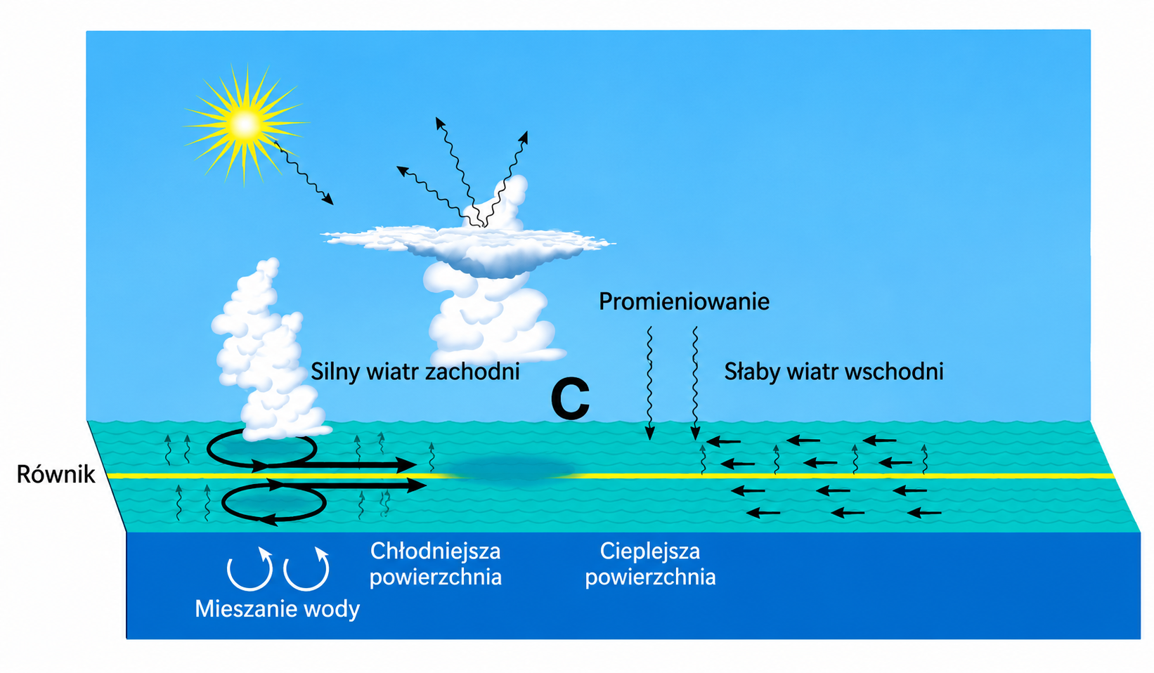
ASCII schematic: storm clouds and strong westerly winds above a cooling ocean surface, with warmer water and weaker easterly winds farther east — **Figure 4. Clouds, wind and ocean interact.** Strong westerly winds blow eastward; weak easterly winds blow westward. C marks converging air. Wavy arrows represent energy exchange, and white arrows in the water represent mixing. The cooler and warmer surface regions are parts of the ASCII mechanism. This conceptual diagram does not show the thermocline or measured wave depth. Polish labels identify strong westerly wind, weak easterly wind, cooler surface, warmer surface and mixing.
Source: Maria Flatau, Piotr J. Flatau, Patricia Phoebus and Pearn P. Niiler (1997), The Feedback between Equatorial Convection and Local Radiative and Evaporative Processes: The Implications for Intraseasonal Oscillations, Journal of the Atmospheric Sciences, 54, 2373–2386, Figure 9c. Graphically reconstructed from the scanned schematic with Polish labels; the original panel label and model abbreviation were omitted. This is a conceptual illustration, not a plot of data.

Local cooling, a change beneath the surface farther east

A westerly wind burst, or several bursts, can generate an oceanic Kelvin wave. It carries a deepening of the thermocline—the layer where temperature falls rapidly with depth—eastward. Colder water is then farther below the surface and cools it less effectively. Local cooling beneath strong winds can therefore accompany later warming farther east.

Surface temperature changes can in turn affect the winds and reinforce the ocean response. This can favour El Niño, but a single wind episode does not determine whether it develops (ocean-response study; the 1997–1998 El Niño).

El Niño and Kelvin waves

El Niño involves warming of the central and eastern equatorial Pacific surface, coupled with changing winds. Warmer water there often accompanies higher sea level. Water expands as it warms, but its distribution also matters: winds and currents change the thickness of the warm upper layer. A raised sea surface can therefore indicate changes beneath the surface, as well as surface warming (NASA explanation).

Kelvin waves help carry these changes eastward. A wave that deepens the thermocline also raises sea level. Colder water lies deeper and cools the surface less effectively, favouring El Niño. During La Niña the central and eastern equatorial Pacific more often shows the opposite pattern: a cooler surface, a shallower thermocline and lower sea level. This is not a lowering of the entire Pacific; warm water may be concentrated more strongly in the west.

The maps compare November 2023, during El Niño, with November 2022, during La Niña. In 2023 a warm equatorial band in the central and eastern Pacific accompanies raised sea level. A year earlier the surface there was cooler, while raised sea level was more apparent in the west. These are not exact mirror images: sea level in 2022 was not below the historical average everywhere. Other ocean changes, including long-term warming and sea-level rise, also contribute. Two monthly snapshots show the contrast between El Niño and La Niña, but cannot trace an individual Kelvin wave.

Four Pacific maps comparing sea-level and surface-temperature anomalies in November 2023 El Niño and November 2022 La Niña — **Figure 5. El Niño and La Niña: surface temperature and sea level.** Panels a–b: November 2023; c–d: November 2022. The upper map in each pair shows sea-level differences in centimetres; the lower shows surface-temperature differences in degrees Celsius. All four use the November average for 1993–2012 as their reference. Warm colours mean above-average values and cool colours below-average values. Each variable has the same scale in both years; end colours also include values beyond the scale. The domain is 120°E–70°W, 30°S–30°N. Dark grey is land; darkest missing-data areas do not mean zero anomaly. Long-term warming and sea-level rise have not been removed. Polish labels read “sea level”, “surface temperature”, “equator” and “November”.
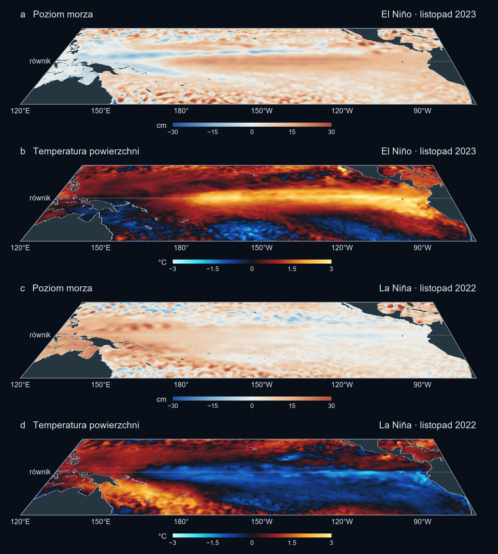
Temperature: NOAA OISST v2.1 monthly means, combining satellite and in-water observations. Sea level: Copernicus Marine SSALTO/DUACS multi-satellite monthly maps, dataset version 202411. These observation-based products interpolate between measurements. For each variable, the average of the 20 Novembers in 1993–2012 was subtracted from November 2023 and 2022. Phase classification: NOAA. Perspective layout and temperature palette adapted from the wind-figure code on the El Niño blog, with new dates, a wider Pacific domain and sea level replacing wind. Wind arrows and the Caribbean box were removed. Land outlines: Natural Earth.

Oceanic Kelvin waves: how disturbances beneath the ocean surface affect climate